Helmholtz EPT with automatically selected kernel
Experimental
Table of contents
Theory
The implemented method is based on Helmholtz EPT, where the estimation of the electric properties consists in the evaluation of the Laplacian of the input map.
The Laplacian of the noisy input map is estimated numerically with a Savitzky-Golay filter [1]. It approximates the map around the voxel of interest with a paraboloid (or a higher order polynomial), of which computes the derivatives. In this way, the Savitzky-Golay filter reduces the impact of noise in the Laplacian computation.
The polynomial fitting on which the Savitzky-Golay filter is based depends on the definition of a kernel of voxels around the voxel of interest. The kernel should be large enough to reduce the noise propagation, but not too large to include voxels from adjacent tissues. In the latter case, the assumption of local homogeneity on which Helmholtz EPT relies would not hold and, therefore, large systematic errors would appear. This implementation of Helmholtz EPT looks automatically for the optimal kernel given a set of options.
In each voxel, the kernel is selected assuring that the estimated properties are physically admissible (i.e., positive conductivity and larger than one permittivity) and that the uncertainty associated with the estimated property value is minimum. The uncertainty is evaluated by propagating it through the fitting under the assumption of independent and identically distributed noise in each voxel of the acquired input map.
References
[1] A. Savitzky and M.J.E. Golay, “Smoothing and differentiation of data by simplified least squares procedures,” Analytical Chemistry, 36(8):1627-39, 1964. DOI: 10.1021/ac60214a047
Settings
Just one input address between tx-sensitivity and trx-phase can be set. If both the addresses are provided, then the complete Helmholtz EPT method will be applied. Otherwise, the approximated method that makes use only of the provided input data will be applied.
Moreover, tx-channel and rx-channel must be equal to 1.
The following specific settings must be configured.
Savitzky-Golay filter
A list of kernels (characterised by the size and the shape) on which the Savitzky-Golay filter can be applied must be provided.
[parameter.savitzky-golay]
    sizes = [[2, 2, 1], [3, 3, 1], [3, 3, 1]]
    shapes = [1, 1, 2]
    degree = 2
    output-index = "example.h5:/index"
sizesis the list of the sizes of the kernels. The size defines the number of voxels along each semi-axis of the kernel. This setting is mandatory.shapesis the list of the shapes of the kernels. The shape is defined according to the following table. This setting is mandatory.degreeis the degree of the interpolating polynomial. It is the same for all the kernels. It must be at least 2 (default:2).output-indexis the address where the map of the selected kernels will be written. It must be a group in an .h5 file. The map contains in each voxel the index of the selected kernel ordered as in thesizesandshapeslists starting from the index 0. Index -1 appears when no kernel is selected. The index map of the electric conductivity, if available, will be written in the group as/electric-conductivity; the index map of the relative permittivity, if available, will be written in the group as/relative-permittivity. If omitted, the map will not be stored.
| Code | Shape | Example with size = [2,2,1] |
|---|---|---|
| 0 | Cross | 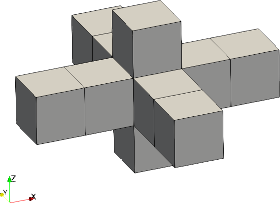 |
| 1 | Ellipsoid | 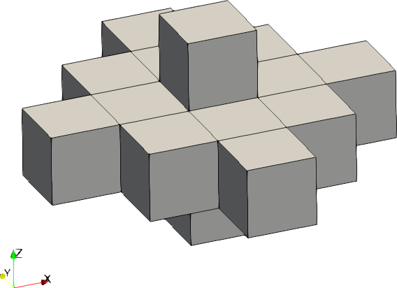 |
| 2 | Cuboid | 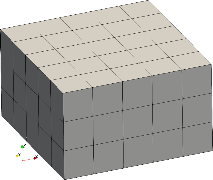 |
Other parameters
[parameter]
    unphysical-values = false
    output-variance = "example.h5:/var"
unphysical-valuesis equal totrueif unphysical values (i.e., negative conductivity and lower than one permittivity) are admitted. (default:false).output-varianceis the address where the variance evaluated for the electric properties will be written. It must be a group in an .h5 file. The variance of the electric conductivity, if available, will be written in the group as/electric-conductivity; the variance of the relative permittivity, if available, will be written in the group as/relative-permittivity. If omitted, the variance will not be stored.
Example
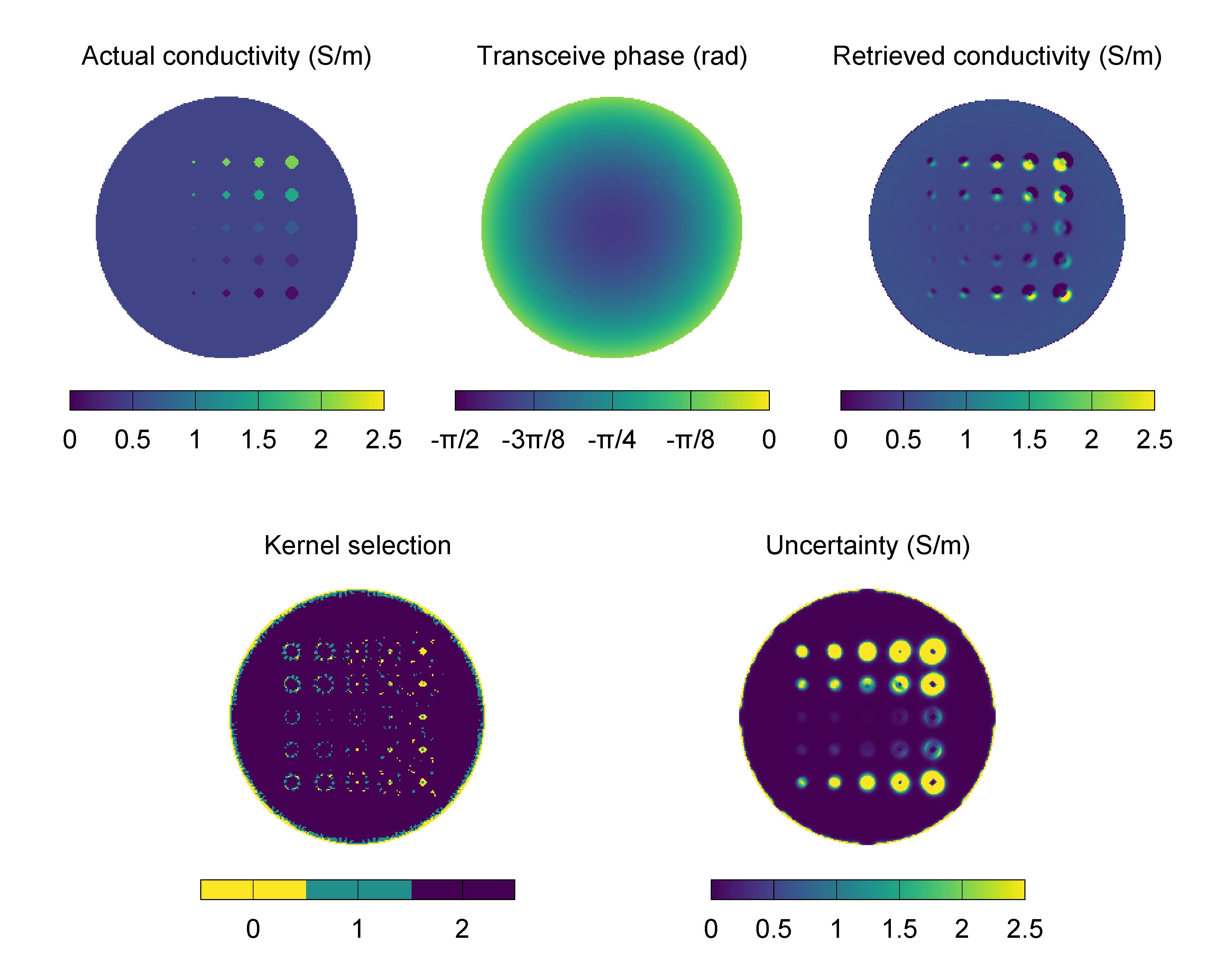
The following configuration file is used to perform the phase-based Helmholtz EPT with automatically selected kernel of a heterogeneous phantom. The input transceive phase has been obtained by simulating the phantom in a birdcage body coil at 64 MHz, that is the Larmor frequency of a 1.5 T scanner.
The configuration file can be downloaded here. The input .h5 file containing the data can be downloaded here.
title = "Example of phase-based Helmholtz EPT with automatically selected kernel"
description = "Heterogeneous phantom imaged at 1.5 T."
method = 100

[mesh]
    size = [200, 200, 11]
    step = [1e-3, 1e-3, 1e-3]

[input]
    frequency = 64e6
    tx-channels = 1
    rx-channels = 1
    trx-phase = 'heterogeneous-phantom-15t.h5:trx_phase'

[output]
    electric-conductivity = 'heterogeneous-phantom-15t-ept-helmholtz-chi2.h5:sigma'

[parameter.savitzky-golay]
    sizes = [[2, 2, 2], [3, 3, 3], [4, 4, 4]]
    shapes = [1, 1, 1]
    output-index = 'heterogeneous-phantom-15t-ept-helmholtz-chi2.h5:index'

[parameter]
    unphysical-values = true
    output-variance = "heterogeneous-phantom-15t-ept-helmholtz-chi2.h5:var"
The retrieved distribution of the electric conductivity is pictured in the following image, together with the expected distribution, the input transceive phase, the selected kernel index and the pixel-wise uncertainty (square root of the electric conductivity pixel-wise variance). Because of the hypothesis of local homogeneity of the electric properties that is at the basis of the Helmholtz EPT method, large errors occur at the boundary of the phantom inclusions. The evaluated variance recognises this error and the automatic system selects smaller kernels near to the boundaries.