Examples
List of examples for each implemented B1-mapping method.
Table of contents
The following examples are based on data simulated of a homogeneous phantom imaged with a birdcage body coil at 64 MHz, that is the Larmor frequency of a 1.5 T scanner.
The .h5 files used in the examples are homogeneous-phantom-15t.h5, containing the geometry of the phantom and the simulated transmit and receive sensitivities, and homogeneous-phantom-15t-prop.h5, containing the physical properties of the phantom.
The description of the imaged body is provided by the .toml file that can be downloaded here.
[body]
    materials = "homogeneous-phantom-15t.h5:/segmentation"
    proton-density = "homogeneous-phantom-15t-prop.h5:/rho"
    longitudinal-relaxation = "homogeneous-phantom-15t-prop.h5:/T1"
    transverse-relaxation = "homogeneous-phantom-15t-prop.h5:/T2"
Double angle
The configuration file for the double angle example can be downloaded here.
title = "Test"
method = 0

[mesh]
    size = [100,100,11]
    step = [2e-3,2e-3,2e-3]

[input]
    body = "phantom.toml"
    tx-sensitivity = "homogeneous-phantom-15t.h5:/tx_sens"
    tx-phase = "homogeneous-phantom-15t.h5:/tx_phase"
    rx-sensitivity = "homogeneous-phantom-15t.h5:/rx_sens"
    rx-phase = "homogeneous-phantom-15t.h5:/rx_phase"

[montecarlo]
    samples = 1
    noise = 0.01

[output]
    alpha-estimate = "homogeneous-phantom-15t-b1map-da.h5:/alpha-est"
    intermediate-images = "homogeneous-phantom-15t-b1map-da.h5:/imgs"

[parameter]
    alpha-nominal = 1.04
    TR = 3000.0
    TE = 0.0
    spoiling = 0.99
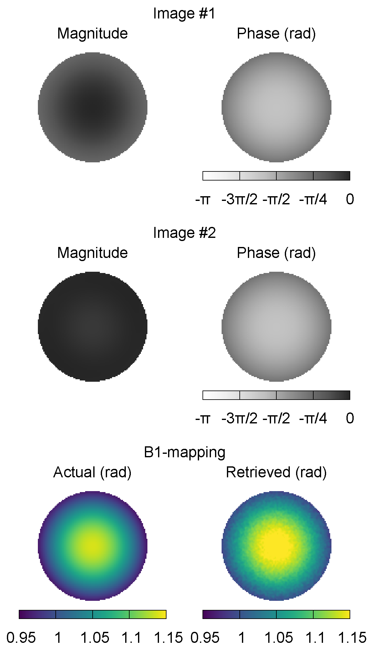
The intermediate images and the actual and the estimated flip-angle are reported in the following picture. The results are obtained by applying the double angle method. Before combining the two intermediate images to obtain the flip-angle estimate, noise with a signal to noise ratio (SNR) equal to 100 is added.
Actual flip-angle
The configuration file for the actual flip-angle example can be downloaded here.
title = "Test"
method = 1

[mesh]
    size = [100,100,11]
    step = [2e-3,2e-3,2e-3]

[input]
    body = "phantom.toml"
    tx-sensitivity = "homogeneous-phantom-15t.h5:/tx_sens"
    tx-phase = "homogeneous-phantom-15t.h5:/tx_phase"
    rx-sensitivity = "homogeneous-phantom-15t.h5:/rx_sens"
    rx-phase = "homogeneous-phantom-15t.h5:/rx_phase"

[montecarlo]
    samples = 1
    noise = 0.01

[output]
    alpha-estimate = "homogeneous-phantom-15t-b1map-afi.h5:/alpha-est"
    intermediate-images = "homogeneous-phantom-15t-b1map-afi.h5:/imgs"

[parameter]
    alpha-nominal = 1.57
    TR = 30.0
    TRratio = 5.0
    TE = 0.0
    spoiling = 0.99
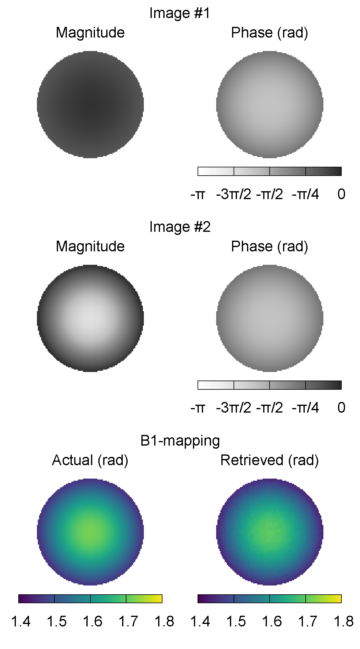
The intermediate images and the actual and the estimated flip-angle are reported in the following picture. The results are obtained by applying the actual flip-angle method. Before combining the two intermediate images to obtain the flip-angle estimate, noise with a signal to noise ratio (SNR) equal to 100 is added.
Bloch–Siegert shift
The configuration file for the Bloch–Siegert shift example can be downloaded here.
title = "Test"
method = 2

[mesh]
    size = [100,100,11]
    step = [2e-3,2e-3,2e-3]

[input]
    body = "phantom.toml"
    tx-sensitivity = "homogeneous-phantom-15t.h5:/tx_sens"
    tx-phase = "homogeneous-phantom-15t.h5:/tx_phase"
    rx-sensitivity = "homogeneous-phantom-15t.h5:/rx_sens"
    rx-phase = "homogeneous-phantom-15t.h5:/rx_phase"

[montecarlo]
    samples = 1
    noise = 0.01

[output]
    alpha-estimate = "homogeneous-phantom-15t-b1map-bss.h5:/alpha-est"
    intermediate-images = "homogeneous-phantom-15t-b1map-bss.h5:/imgs"

[parameter]
    alpha-nominal = 1.57
    TR = 30.0
    TE = 0.0
    spoiling = 0.99
    bss-offres = 4.0
    bss-length = 8.0
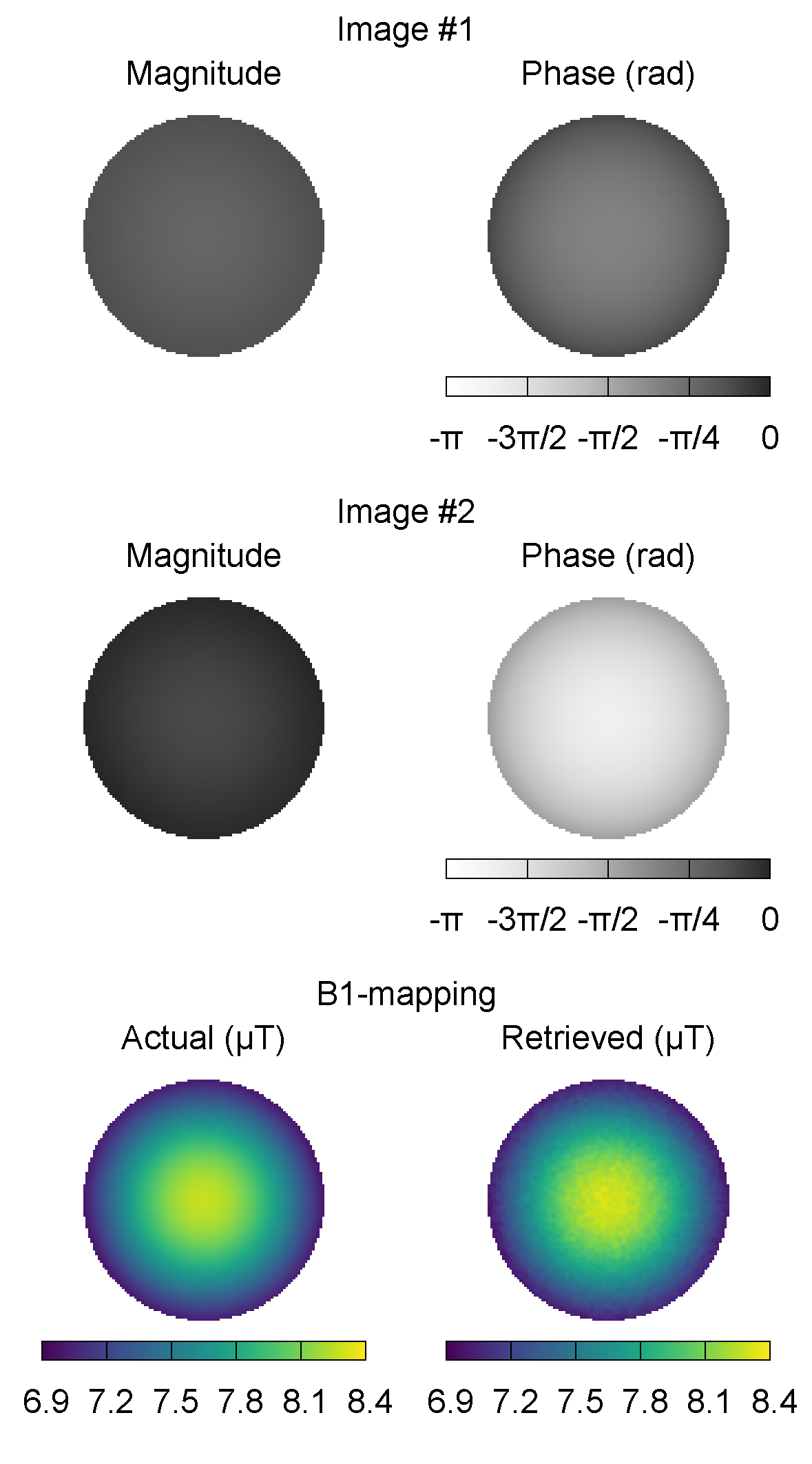
The intermediate images and the actual and the estimated transmit sensitivity magnitude are reported in the following picture. The results are obtained by applying the Bloch–Siegert shift method. Before combining the two intermediate images to obtain the transmit sensitivity magnitude estimate, noise with a signal to noise ratio (SNR) equal to 100 is added.
Transceive phase acquisition
The configuration file for the transceive phase acquisition example can be downloaded here.
title = "Test"
method = 3

[mesh]
	size = [100,100,11]
	step = [2e-3,2e-3,2e-3]

[input]
	body = "phantom.toml"
	tx-sensitivity = "homogeneous-phantom-15t.h5:/tx_sens"
	tx-phase = "homogeneous-phantom-15t.h5:/tx_phase"
    rx-sensitivity = "homogeneous-phantom-15t.h5:/rx_sens"
	rx-phase = "homogeneous-phantom-15t.h5:/rx_phase"

[montecarlo]
	samples = 1
	noise = 0.01

[output]
	alpha-estimate = "homogeneous-phantom-15t-b1map-trx.h5:/trx-phase"
	intermediate-images = "homogeneous-phantom-15t-b1map-trx.h5:/imgs"

[parameter]
	alpha-nominal = 1.57
	TR = 30.0
	TE = 0.0
	spoiling = 0.99
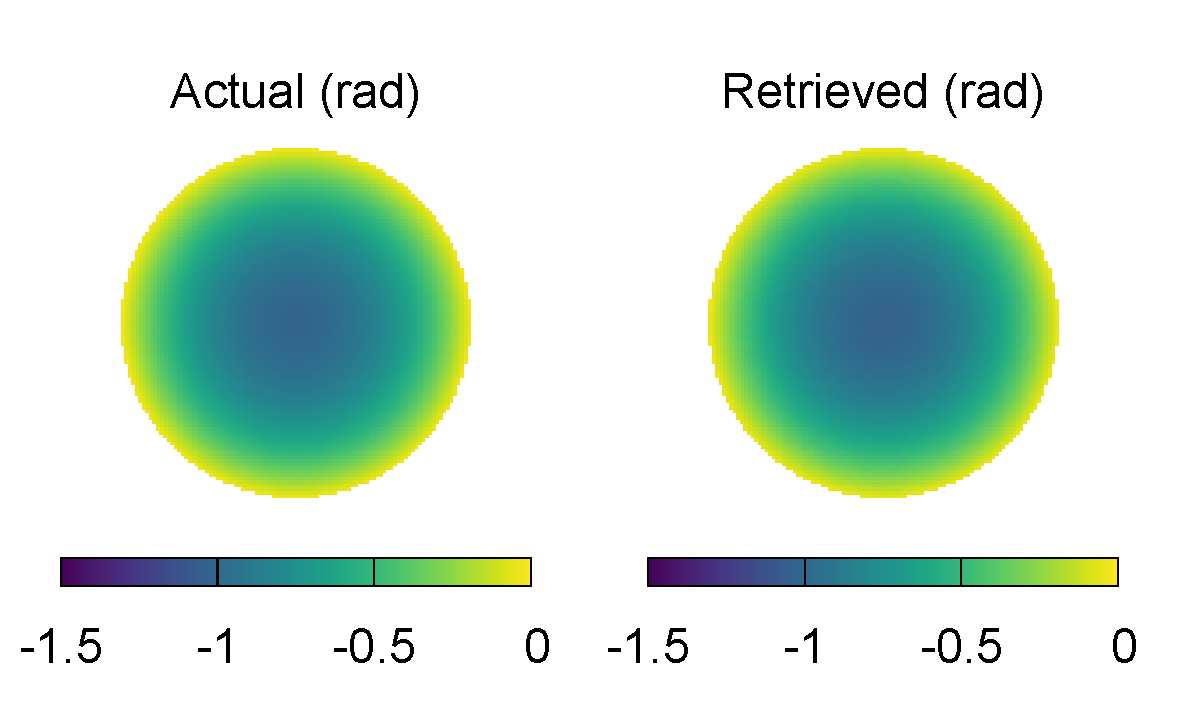
The actual and the estimated transceive phase are reported in the following picture. Noise with a signal to noise ratio (SNR) equal to 100 is simulated.