Convection-reaction EPT

Particularly effective method when applied on only transceive phase maps. It requires that the input is acquired near the mid-plane of a birdcage-like coil.

Theory
Settings
Example

Theory

A brief introduction to convection-reaction EPT is provided below. More details can be found in [1].

Complete method

For biological tissues, whose magnetic permeability can be reasonably assumed constant and equal to the one of vacuum $\mu_0$, the following equation for a time-harmonic magnetic field ${\bf H}$ holds, $$ \nabla\times\left(\tilde{\varepsilon}^{-1} \nabla\times{\bf H} \right) = \omega^2\mu_0{\bf H}\,. $$ In the latter, $\omega$ is the angular frequency of the electromagnetic radiation (i.e., the Larmor angular frequency) and $\tilde{\varepsilon} = \varepsilon_{\rm r} \varepsilon_0 - {\rm i} \sigma/\omega$ is the complex permittivity, which is defined by means of the vacuum permittivity $\varepsilon_0$ and of the two electric properties: the relative permittivity $\varepsilon_{\rm r}$ and the electric conductivity $\sigma$.

By introducing the unknown variable $\gamma = \tilde{\varepsilon}^{-1}$, the previous equation can be rewritten as $$ \nabla \gamma \times \left(\nabla \times {\bf H}\right) - \gamma \nabla^2 {\bf H} = \omega^2 \mu_0 {\bf H}\,. $$ Under the hypothesis of a negligible gradient $\nabla H_z \simeq 0$, which is verified around the mid-plane of a birdcage-like coil, the $x$ and $y$ components of the latter equation can be combined according to the rotating component associated to the complex transmit sensitivity ($B_1^+ = \mu_0 H^+$), where $$ H^+ = \frac{H_x + {\rm i} H_y}{2}\,. $$ This leads to the convection-reaction equation with respect to the unknown $\gamma$, here written in conservative form, $$ \boxed{ \nabla \cdot \left( \gamma {\bf v}^+ \right) = -\omega^2 \mu_0 B_1^+ }\,, $$ where ${\bf v}^+ = \nabla B_1^+ - {\rm i} \nabla \times \left( B_1^+ \hat{z} \right)$. An equivalent formulation is derived in [2].

The convection-reaction problem is solved with the finite difference scheme, but the method is often unstable. It is possible to improve the results by introducing an artificial diffusion term such that the equation becomes $$ -\lambda \nabla^2 \gamma + \nabla \cdot \left( \gamma {\bf v}^+ \right) = -\omega^2 \mu_0 B_1^+\,, $$ where $\lambda$ is the diffusion coefficient, as described in [3].

To solve the equation, boundary conditions must be provided. Precisely, an estimate of the value of $\gamma$ on the boundary is set.

Two-dimensional approximation

Since the hypothesis of a negligible gradient $\nabla H_z \simeq 0$ holds only around the mid-plane of the birdcage-like coil, the computational domain could be too thin to reasonably force the value of $\gamma$ on the boundaries perpendicular to the longitudinal direction.

For this reason and in order to reduce the computational cost of the method, a two-dimensional approximated equation can be obtained by assuming that the properties are almost constant along the longitudinal direction (i.e., $\partial_z \gamma \simeq 0$). In this case, the convection-reaction equation is $$ \boxed{ \nabla_{xy} \cdot \left( \gamma {\bf v}_{xy}^+ \right) + \gamma \frac{\partial^2 B_1^+}{\partial z^2} = -\omega^2 \mu_0 B_1^+ }\,, $$ where ${\bf v}_{xy}^+ = (v, {\rm i} v)$ and $v = \partial_x B_1^+ - {\rm i} \partial_y B_1^+$.

Similarly to the three-dimensional case, also this equation can be solved numerically with the addition of an artificial diffusion term in order to stabilize the method.

Phase-based approximation

Analogously to the complete equation obtained for the transmit sensitivity $B_1^+$, the equation $$ \nabla \cdot \left( \gamma {\bf v}^- \right) = -\omega^2 \mu_0 B_1^-\,, $$ holds with ${\bf v}^- = \nabla B_1^- + {\rm i} \nabla \times \left( B_1^- \hat{z} \right)$, $B_1^- = \mu_0 H^-$ the complex receive sensitivity and $$ H^- = \frac{H_x - {\rm i} H_y}{2}\,. $$

It is worth noting that also the longitudinal component of the receive field should be almost constant in the region of interest. This can be obtained, for example, operating also in reception near the mid-plane of a birdcage-like coil. In this case, it is reasonable to assume that for both the transmit and the receive sensitivities, $\nabla \vert B_1^+ \vert \simeq 0$ and $\nabla \vert B_1^- \vert \simeq 0$.

Thus, denoting by $\varphi^+$ the phase of the transmit sensitivity the former equation can be approximated as $$ \nabla \cdot \left( \gamma {\bf v}_\varphi^+ \right) + {\rm i} \gamma \vert \nabla \varphi^+ \vert^2 = {\rm i} \omega^2 \mu_0\,, $$ where ${\bf v}^+_{\varphi} = \nabla \varphi^+ - {\rm i} \nabla \times \left( \varphi^+ \hat{z} \right)$.

Similarly, the latter equation can be approximated as $$ \nabla \cdot \left( \gamma {\bf v}_\varphi^- \right) + {\rm i} \gamma \vert \nabla \varphi^- \vert^2 = {\rm i} \omega^2 \mu_0\,, $$ where $\varphi^-$ denotes the phase of the receive sensitivity and ${\bf v}^-_{\varphi} = \nabla \varphi^- + {\rm i} \nabla \times \left( \varphi^- \hat{z} \right)$.

The so-called transceive phase $\varphi^{\pm} = \varphi^+ + \varphi^-$, which is the phase that can be actually measured with MRI scans, appears when the two equations are added up. Moreover, if $\sigma \gg \omega \varepsilon$ (this inequality is true for almost all biological tissues at frequencies up to 128 MHz, that is the Larmor frequency of a 3 T scanner), the imaginary part of the sum equation is $$ \boxed{ \nabla \cdot \left( \rho \nabla \varphi^{\pm} \right) = 2 \omega \mu_0 }\,, $$ where $\rho = \sigma^{-1}$ is the unknown electric resistivity of the biological tissues.

This equation can be solved with a stable numerical method based on an upwind finite difference scheme. Anyway, it is possible to introduce an artificial diffusion term as a further stabilization.

Moreover, as well as the complex equation, also in this case the problem can be approximated in two dimensions assuming that the electric resistivity is almost constant along the longitudinal direction (i.e., $\partial_z \rho \simeq 0$). The resulting two-dimensional convection-reaction equation in conservative form is $$ \boxed{ \nabla_{xy} \cdot \left( \rho \nabla_{xy} \varphi^{\pm} \right) + \rho \frac{\partial^2 \varphi^{\pm}}{\partial z^2} = 2 \omega \mu_0 }\,. $$

The phase-based approximation of the convection-reaction EPT is derived in [4].

Derivatives estimation

Provided a noisy measurement of the distribution of $B_1^+$, or $\varphi^{\pm}$, its derivatives can be estimated with a second-order Savitzky-Golay filter [5]. It approximates the distribution around the voxel of interest with a paraboloid, of which computes the derivatives. In this way, the Savitzky-Golay filter reduces the impact of noise in the derivatives computation.

Current implementations of the complete complex-valued method (and its two-dimensional approximation) are numerically unstable and most of the time leads to wrong reconstructions. The phase-based approximation, instead, is stable and provides good results.

References

[1] A. Arduino, “Mathematical methods for magnetic resonance based electric properties tomography,” PhD thesis, Politecnico di Torino, 2018. DOI: 10.6092/polito/porto/2698325

[2] F.S. Hafalir, O.F. Oran, N. Gurler and Y.Z. Ider, “Convection-reaction equation based magnetic resonance electrical properties tomography (cr-MREPT),” IEEE Transactions on Medical Imaging, 33(3):777–93, 2014. DOI: 10.1109/TMI.2013.2296715.

[3] C. Li, W. Yu and S.Y. Huang, “An MR-based viscosity-type regularization method for electrical properties tomography,” Tomography, 3(1), 2017. DOI: 10.18383/j.tom.2016.00283

[4] N. Gurler and Y.Z. Ider, “Gradient-based electrical conductivity imaging using MR phase,” Magnetic Resonance in Medicine, 77(1):137–50, 2017. DOI: 10.1002/mrm.26097.

[5] A. Savitzky and M.J.E. Golay, “Smoothing and differentiation of data by simplified least squares procedures,” Analytical Chemistry, 36(8):1627-39, 1964. DOI: 10.1021/ac60214a047

Settings

The trx-phase input address is mandatory, whereas tx-sensitivity can be omitted. If both the addresses are provided, then the complete convection-reaction EPT method will be applied. Otherwise, the phase-based approximated method will be applied.

Moreover, tx-channel and rx-channel must be equal to 1.

The following specific settings must be configured.

Savitzky-Golay filter

The Savitzky-Golay filter can be applied on kernels with different size and shape.

[parameter.savitzky-golay]
    size = [2, 2, 1]
    shape = 0
    degree = 2
    weight-param = 0.05

size is the number of voxels along each semi-axis of the kernel (default: [1,1,1]).
shape selects the kernel shape according to the following table (default: 0).
degree is the degree of the interpolating polynomial. It must be at least 2 (default: 2).
weight-param is a parameter of the weight function used for the reference image. It is used only if a reference image is provided in input (default: 0.05).

Code	Shape	Example with `size = [2,2,1]`
0	Cross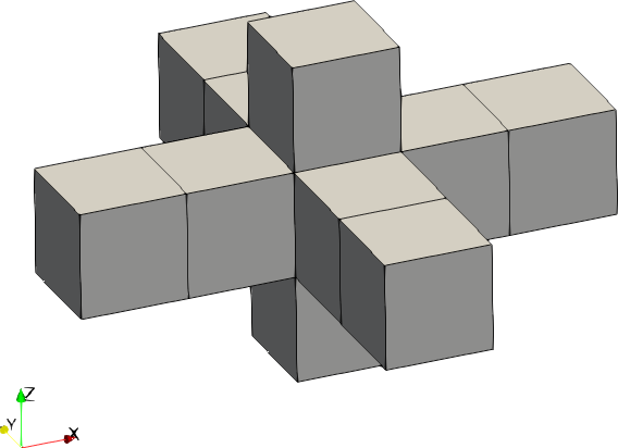
1	Ellipsoid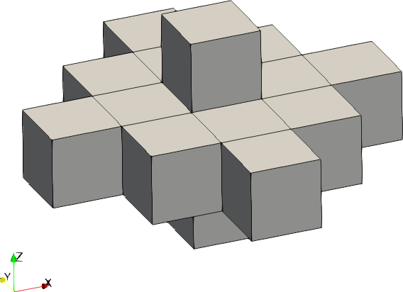
2	Cuboid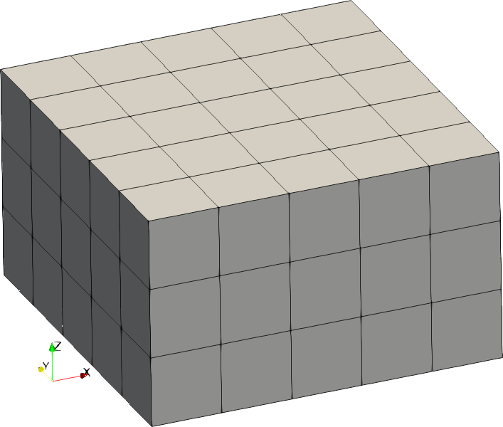

If a reference image is provided in input to the method, the Savitzky-Golay filter is anatomically adapted with respect to it. Precisely, in the filter procedure each voxel contribution is weighted according to a Gaussian of standard deviation weight-param applied to the relative contrast with respect to the central voxel.

Boundary condition

The boundary condition set the value of the electric properties at the boundary of the domain.

[parameter.dirichlet]
    electric-conductivity = 0.1 # [S/m]
    relative-permittivity = 50.0

electric-conductivity is the value of the electric conductivity forced at the boundary in siemens per meter (default: 0.0).
relative-permittivity is the value of the relative permittivity forced at the boundary (default: 1.0).

The boundary conditions are applied at the interface between tissue and air. The implemented algorithm identifies as air all the voxels in which the input quantity is Not-a-Number, so, before running CR-EPT on your data, take care to set all the voxels in air to Not-a-Number.

Other parameters

[parameter]
    volume-tomography = false
    imaging-slice = 3
    artificial-diffusion = true
    artificial-diffusion-coefficient = 0.1
	max-iterations = 1000
	tolerance = 1e-6

volume-tomography is equal to true to solve the three-dimensional problem; otherwise, for the two-dimensional approximation, it is equal to false (default: false).
imaging-slice is the index of the slice on which the two-dimensional tomography will be performed. It must be set only if volume-tomography is false (default: the index of the mid-plane).
artificial-diffusion is equal to true to add the artificial diffusion term to stabilize the problem; otherwise it is equal to false (default: false).
artificial-diffusion-coefficient is equal to the value of the artificial diffusion coefficient expressed in tesla (for the complete case) or in radian (for the phase-based approximation). It must be set only if artificial-diffusion is true (default: 0.0).
max-iterations is equal to the maximum number of iterations the BiCGStab iterative method will perform to solve the linear system of equations obtained by discretizing the CR-EPT equation (default: 1000).
tolerance is the tolerance of the BiCGStab iterative solver; the iterations are stopped once a residual equal to or lower than the tolerance is reached (default: 1e-6).

Example

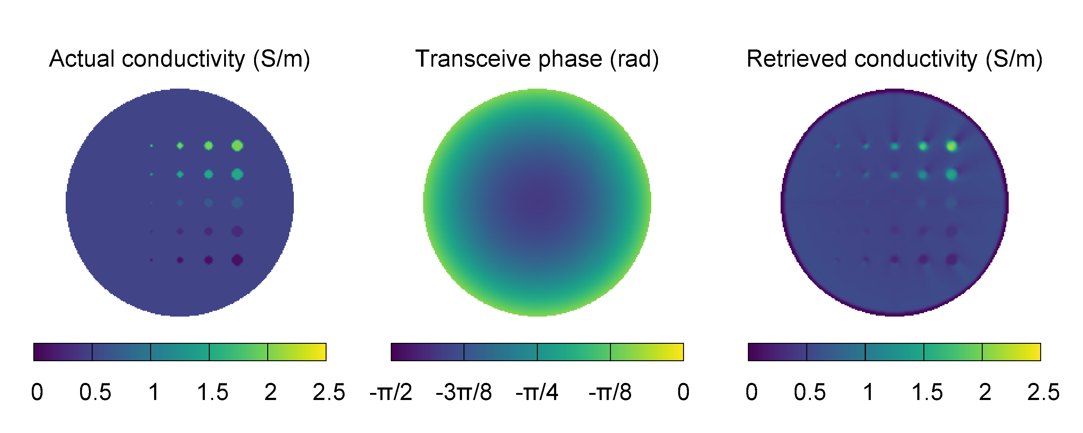
The following configuration file is used to perform the phase-based approximated convection-reaction EPT of a heterogeneous phantom. The input transceive phase has been obtained by simulating the phantom in a birdcage body coil at 64 MHz, that is the Larmor frequency of a 1.5 T scanner.

The configuration file can be downloaded here. The input .h5 file containing the data can be downloaded here.

title = "Example of convection-reaction EPT"
description = "Heterogeneous phantom imaged at 1.5 T. Phase-based approximation."
method = 1

[mesh]
    size = [200, 200, 11]
    step = [1e-3, 1e-3, 1e-3]

[input]
    frequency = 64e6
    tx-channels = 1
    rx-channels = 1
#   tx-sensitivity = 'heterogeneous-phantom-15t.h5:tx_sens'
    trx-phase = 'heterogeneous-phantom-15t.h5:trx_phase'

[output]
    electric-conductivity = 'heterogeneous-phantom-15t-ept-convreact.h5:sigma'
#   relative-permittivity = 'heterogeneous-phantom-15t-ept-convreact.h5:epsr'

[parameter.savitzky-golay]
    size = [1, 1, 1]
    shape = 0
[parameter.dirichlet]
    electric-conductivity = 0.01
#   relative-permittivity = 1.0
[parameter]
    volume-tomography = false
    imaging-slice = 5
    artificial-diffusion = true
    artificial-diffusion-coefficient = 5e-3

The retrieved distribution of the electric conductivity is pictured in the following image, together with the expected distribution and the input transceive phase. Despite the guess of the Dirichlet boundary condition on the electric conductivity was wrong, it plays a role only near the boundary itself because of the artificial diffusion. The recovery in the inner regions of the phantom is practically unaffected by the boundary condition.