Gradient EPT

EPT method for parallel transmission imaging systems. It requires that the input is acquired near the mid-plane of a longitudinally symmetric transmit coil.

Theory
Settings
Example

Theory

A brief introduction to gradient EPT is provided below. More details can be found in [1].

First step (local estimation)

Gradient EPT is built on top of the same equation of convection-reaction EPT repeated for each transmit channel of the parallel transmission system. Thus, it relies on the same hypothesis of convection-reaction EPT: the gradient of $\nabla H_{i,z} \simeq 0$ is negligible for any transmit channel $i$. This assumption is verified any time the RF coil is longitudinally symmetric, which is very often the case for volume coils.

For convenience, the convection-reaction EPT equation is rewritten, for the $i$-th transmit channel, as $$ \omega^2 \mu_0 B_{1,i}^+ \tilde{\varepsilon} + \nabla^2 B_{1,i}^+ = \nabla B_{1,i}^+ \cdot \left( g_+, -{\rm i} g_+, g_z \right)\,, $$ where $g_+ = g_x + {\rm i} g_y$ and ${\bf g} = \nabla \log(\tilde{\varepsilon})$.

The problem with parallel transmission is that, in general, it is impossible to estimate the complex transmit sensitivity $B_{1,i}^+$, because there is no way to deduce the phase of the $i$-th transmit sensitivity $\varphi^+_i$ from the measured transceive phase $\varphi^\pm_i = \varphi^+_i + \varphi^-$, which entangles $\varphi^+_i$ with the phase of the receive sensitivity $\varphi^-$.

However, being the receive sensitivity the same in all the acquired transceive phases, it is possible to estimate the relative phases as $$ \varphi_i^{+,{\rm r}} = \varphi_i^\pm - \varphi_0^\pm = \varphi_i^+ - \varphi_0^+\,, $$ where $\varphi_0^+$ has been chosen as the reference phase. Thus, the $i$-th complex transmit sensitivity can be written as $$ B_{1,i}^+ = B_{1,i}^{+,{\rm r} } {\rm e}^{ {\rm i} \varphi_0^+ }\,, $$ where $B_{1,i}^{+,{\rm r} } = \vert B_{1,i}^+ \vert {\rm e}^{ {\rm i}\varphi_i^{+,{\rm r} } }$ is the measurable part.

Thus, the starting equation can be elaborated by splitting the measurable and the unknown parts of the complex transmit sensitivity to obtain $$ \boxed{ -{\rm i} 2 \nabla B_{1,i}^{+,{\rm r} } \cdot \nabla \varphi_0^+ + \nabla B_{1,i}^{+,{\rm r} } \cdot \left( g_+, -{\rm i} g_+, g_z \right) + B_{1,i}^{+,{\rm r} } \vartheta^+ = \nabla^2 B_{1,i}^{+,{\rm r} } }\,, $$ where $\nabla \varphi_0^+$, $g_+$, $g_z$ and $\vartheta^+$ are treated as algebraically independent unknowns. In particular, $\vartheta^+ = -\omega^2 \mu_0 \tilde{\varepsilon} + \vert \nabla \varphi_0^+ \vert^2 - {\rm i} \nabla^2 \varphi_0^+ + {\rm i} \nabla \varphi_0^+ \cdot \left( g_+, -{\rm i} g_+, g_z \right)$ collects all the non-linear unknown terms and its combination with the other unknown allows retrieving a first estimate of the electric properties $\tilde{\varepsilon}$.

The latter equation is solved in a voxel-by-voxel fashion by combining its evaluations for each transmit channel in a linear system. The linear system is solved as many times as the number of transmit channels, every time using a different channel for the reference phase. The results, weighted by the magnitude of the transmit sensitivity of the reference channel, are then averaged to reduce the effect of numerical errors, as described in [2].

Second step (global estimation)

The solution of the previous system of equations provides in each voxel a first local estimate of the electric properties $\tilde{\varepsilon}_0$ as well as an estimate of the derivatives of its logarithm $g_{+,0}$ and $g_{z,0}$.

The retrieved distributions of the derivatives can be elaborated to provide a global estimate of the electric properties. In the EPTlib application, the global estimate is obtained by solving the minimisation problem $$ \boxed{ \tilde{\varepsilon} = {\rm argmin} \left( \left\vert g_+(\tilde{\varepsilon}) - g_{+,0} \right\vert^2 + \left\vert g_z(\tilde{\varepsilon}) - g_{z,0} \right\vert^2 \right) }\,. $$ The minimisation is performed by solving the associated linear Euler equation with the finite element method (FEM).

The problem can be solved with a seed point constraint, where given values of $\tilde{\varepsilon}$ are constrained in some selected voxels, referred to as seed points. Otherwise, the problem can be solved with an additive regularization term which forces the distribution of $\tilde{\varepsilon}$ to be similar to $\tilde{\varepsilon}_0$ in some regions [3].

Other techniques, like the ones described in [4], can be used, but they are not implemented in EPTlib, yet.

Two-dimensional approximation

In order to reduce the computational cost of the method, a two-dimensional approximated equation can be obtained by assuming that the properties are almost constant along the longitudinal direction (i.e., $g_z \simeq 0$) as well as the reference phase (i.e., $\partial_z \varphi_0^+ \simeq 0$). In this case, the equation for the local estimate is $$ \boxed{ -{\rm i} 2 \nabla_{xy} B_{1,i}^{+,{\rm r} } \cdot \nabla_{xy} \varphi_0^+ + \nabla_{xy} B_{1,i}^{+,{\rm r} } \cdot \left( g_+, -{\rm i} g_+ \right) + B_{1,i}^{+,{\rm r} } \vartheta_{xy}^+ = \nabla^2 B_{1,i}^{+,{\rm r} } }\,, $$ with $\vartheta_{xy}^+ = -\omega^2\mu_0 \tilde{\varepsilon} + |\nabla_{xy} \varphi_0^+ |^2 - {\rm i} \nabla_{xy}^2 \varphi_0^+ + {\rm i} \nabla_{xy} \varphi_0^+ \cdot (g_+, -{\rm i}g_+)$.

In this case, also the global estimate is performed in two dimensions by solving the minimisation problem $$ \boxed{ \tilde{\varepsilon} = {\rm argmin}\ \left\vert g_+(\tilde{\varepsilon}) - g_{+,0} \right\vert^2 }\,, $$ with the constraint provided by seed points or the additive regularization term. In the latter equation, $g_{+,0}$ denotes the estimate of the derivative obtained by solving the previous linear system pixel-by-pixel.

Derivatives estimation

Provided a noisy measurement of the distribution of $B_1^+$, or $\varphi^{\pm}$, its derivatives can be estimated with a second-order Savitzky-Golay filter [5]. It approximates the distribution around the voxel of interest with a paraboloid, of which computes the derivatives. In this way, the Savitzky-Golay filter reduces the impact of noise in the derivatives computation.

References

[1] A. Arduino, “Mathematical methods for magnetic resonance based electric properties tomography,” PhD thesis, Politecnico di Torino, 2018. DOI: 10.6092/polito/porto/2698325

[2] J. Liu, X. Zhang, S. Schmitter, P.-F. Van de Moortele and B. He, “Gradient-based electrical properties tomography (gEPT): a robust method for mapping electrical properties of biological tissues in vivo using magnetic resonance imaging,” Magnetic Resonance in Medicine, 74(3):634-46, 2015. DOI: 10.1002/mrm.25434

[3] J. Liu, Q. Shao, Y. Wang, G. Adriany, J. Bischof, P.-F. Van de Moortele and B. He, “In vivo imaging of electrical properties of an animal tumor model with an 8-channel transceiver array at 7 T using electrical properties tomography,” Magnetic Resonance in Medicine, 78(6):2157-69, 2017. DOI: 10.1002/mrm.26609

[4] Y. Wang, P.-F. Van de Moortele and B. He, “CONtrast Conformed Electrical Properties Tomography (CONCEPT) based on multi-channel transmission and alternating direction method of multipliers,” IEEE Transactions on Medical Imaging, 38(2):349-59, 2019. DOI: 10.1109/TMI.2018.2865121

[5] A. Savitzky and M.J.E. Golay, “Smoothing and differentiation of data by simplified least squares procedures,” Analytical Chemistry, 36(8):1627-39, 1964. DOI: 10.1021/ac60214a047

Settings

Both the input addresses are mandatory.

tx-channel must be at least equal to 5.

rx-channel must be equal to 1.

The following specific settings must be configured.

Savitzky-Golay filter

The Savitzky-Golay filter can be applied on kernels with different size and shape.

[parameter.savitzky-golay]
    size = [2, 2, 1]
    shape = 0
    degree = 2
    weight-param = 0.05

size is the number of voxels along each semi-axis of the kernel (default: [1,1,1]).
shape selects the kernel shape according to the following table (default: 0).
degree is the degree of the interpolating polynomial. It must be at least 2 (default: 2).
weight-param is a parameter of the weight function used for the reference image. It is used only if a reference image is provided in input (default: 0.05).

Code	Shape	Example with `size = [2,2,1]`
0	Cross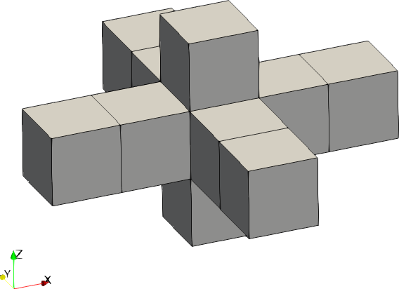
1	Ellipsoid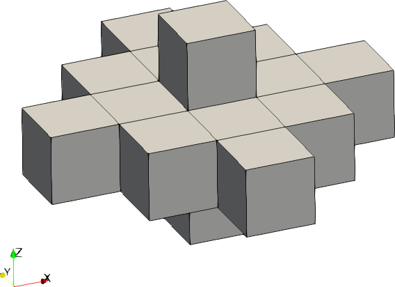
2	Cuboid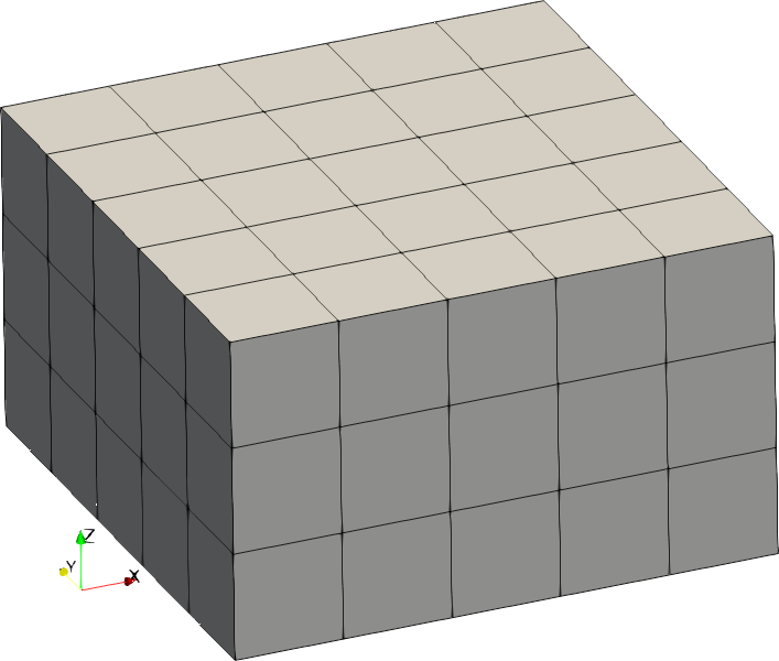

If a reference image is provided in input to the method, the Savitzky-Golay filter is anatomically adapted with respect to it. Precisely, in the filter procedure each voxel contribution is weighted according to a Gaussian of standard deviation weight-param applied to the relative contrast with respect to the central voxel.

Seed points

The seed points are used only if the full run of gradient EPT is executed.

[parameter.seed-point]
    use-seed-point = true
    coordinates = [[15, 20, 25], [25, 20, 15]]
    electric-conductivity = [0.1, 0.2] # [S/m]
    relative-permittivity = [50.0, 70.0]

use-seed-point is equal to true if seed points are used for inverting the gradient (default: false).
coordinates is the list of the integer coordinates of the voxels where the seed points are set. This setting is mandatory if use-seed-point is true, otherwise it is ignored.
electric-conductivity is the list of the values of the electric conductivity forced in the seed points in siemens per meter. This setting is mandatory if use-seed-point is true, otherwise it is ignored.
relative-permittivity is the list of the values of the relative permittivity forced in the seed points. This setting is mandatory if use-seed-point is true, otherwise it is ignored.

Regularization

If the seed point is not used, the gradient is inverted with regularization based on the local estimation of the electric properties.

[parameter.regularization]
    regularization-coefficient = 1e-3
    gradient-tolerance = 0.1
    output-mask = "example.h5:/mask"

regularization-coefficient set the regularization coefficient in unit per square meter (default: 1.0).
gradient-tolerance set the relative tolerance with respect to the maximum gradient for the determination of the homogeneous regions (default: 0.0).
output-mask is the address where the homogeneous regions mask will be written. It must be a dataset in an .h5 file. If omitted, the mask will not be stored.

Other parameters

[parameter]
    volume-tomography = false
    imaging-slice = 3
    full-run = true
    output-gradient = "example.h5:/grad"

volume-tomography is equal to true to solve the three-dimensional problem, otherwise, for the two-dimensional approximation, it is equal to false (default: false).
imaging-slice is the index of the slice on which the two-dimensional tomography will be performed. It must be set only if volume-tomography is false (default: the index of the mid-plane).
full-run is equal to true to execute the full run of gradient EPT; otherwise, it is equal to false to stop the execution after the first local estimate of the electric properties (default: true). This feature is useful in experimenting with the method implementation. It will probably be removed in a future release of the software.
output-gradient is the address where the gradient computed in the local step will be written. It must be a group in an .h5 file. Real and imaginary part of $g_{+,0}$ will be written in the group as /gplus/real and /gplus/imag, respectively. If also $g_{z,0}$ is computed, it will be written in the group as /gz/real and /gz/imag. If omitted, the gradient will not be stored.

Example

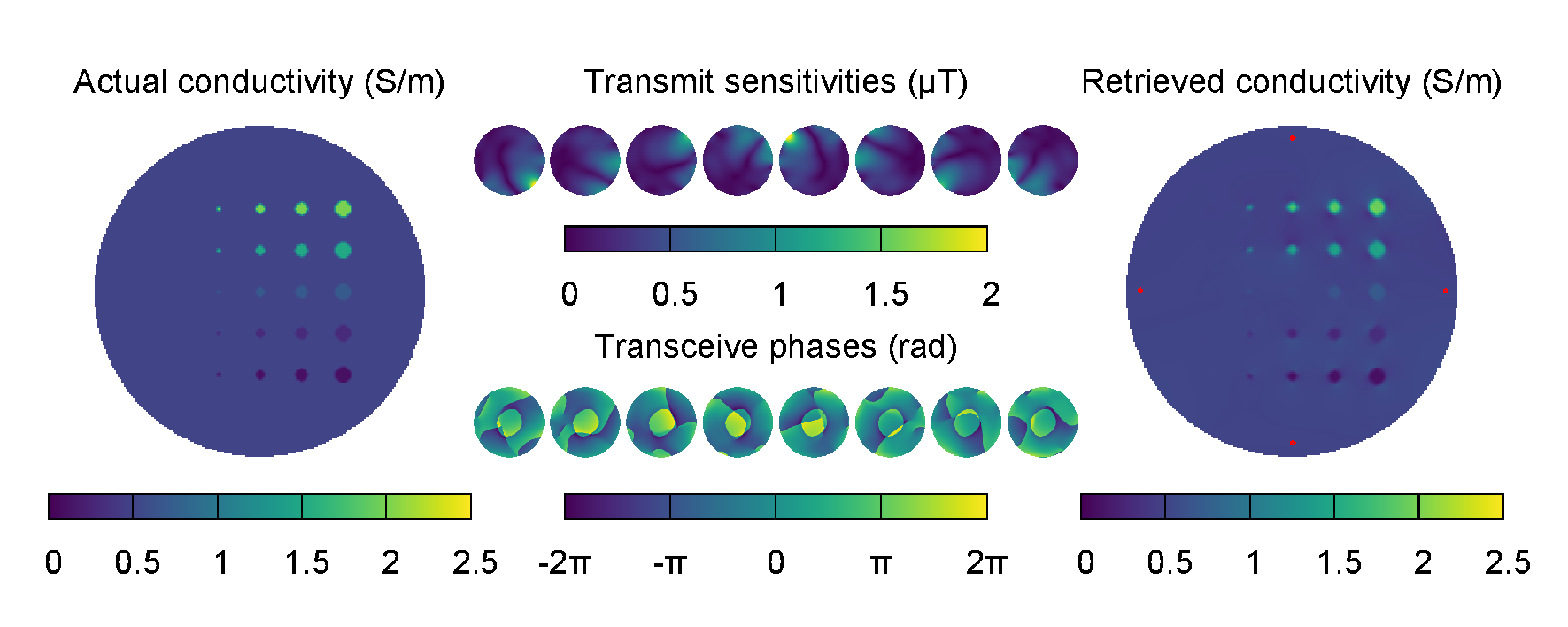
The following configuration file is used to perform the gradient EPT of a heterogeneous phantom. The input transmit sensitivities and transceive phases have been obtained by simulating the phantom in a volume coil designed for parallel transmission at 297 MHz, that is the Larmor frequency of a 7 T scanner. The same coil has been used in reception with a circular polarization.

The configuration file can be downloaded here. The input .h5 file containing the data can be downloaded here.

title = "Example of gradient EPT"
description = "Heterogeneous phantom imaged at 7 T in pTx."
method = 2

[mesh]
    size = [200, 200, 11]
    step = [1e-3, 1e-3, 1e-3]

[input]
    frequency = 297e6
    tx-channels = 8
    rx-channels = 1
    tx-sensitivity = 'heterogeneous-phantom-7t-ptx.h5:channels/>/tx_sens'
    trx-phase = 'heterogeneous-phantom-7t-ptx.h5:channels/>/trx_phase'

[output]
    electric-conductivity = 'heterogeneous-phantom-7t-ptx-ept-gradient.h5:sigma'
    relative-permittivity = 'heterogeneous-phantom-7t-ptx-ept-gradient.h5:epsr'

[parameter.savitzky-golay]
    size = [1, 1, 1]
    shape = 0
[parameter]
    volume-tomography = false
    imaging-slice = 5
    full-run = true
[parameter.seed-point]
    use-seed-point = true
    coordinates = [[100, 10, 5], [10, 100, 5], [100, 190, 5], [190, 100, 5], ]
    electric-conductivity = [0.5, 0.5, 0.5, 0.5, ]
    relative-permittivity = [80.0, 80.0, 80.0, 80.0, ]

The retrieved distribution of the electric conductivity is pictured in the following image, together with the expected distribution and the input maps. In order to determine the seed points (pictured in the output map with small red dots), it has been assumed that the properties of the phantom background were known.