Helmholtz EPT
Fast method with very few requirements on its input. It produces large errors at the boundary between biological tissues with different electric properties.
Table of contents
Theory
A brief introduction to Helmholtz EPT is provided below. More details can be found in [1].
Complete method
For biological tissues, whose magnetic permeability can be reasonably assumed constant and equal to the one of vacuum \(\mu_0\), the following equation for a time-harmonic magnetic field \({\bf H}\) holds, $$ \nabla\times\left(\tilde{\varepsilon}^{-1} \nabla\times{\bf H} \right) = \omega^2\mu_0{\bf H}\,. $$ In the latter, \(\omega\) is the angular frequency of the electromagnetic radiation (i.e., the Larmor angular frequency) and \(\tilde{\varepsilon} = \varepsilon_{\rm r} \varepsilon_0 - {\rm i} \sigma/\omega\) is the complex permittivity, which is defined by means of the vacuum permittivity \(\varepsilon_0\) and of the two electric properties: the relative permittivity \(\varepsilon_{\rm r}\) and the electric conductivity \(\sigma\).
In regions where the electric properties are almost homogeneous (like within a biological tissue), the previous equation can be elaborated to provide the Helmholtz equation $$ -\nabla^2 H_i = \omega^2 \mu_0 \tilde{\varepsilon} H_i\,, $$ which holds for any Cartesian component \(i = x\), \(y\), or \(z\). Moreover, thanks to the linearity of the Helmholtz equation with respect to \({\bf H}\), it holds also for the two rotating components associated to the complex transmit (\(B_1^+ = \mu_0 H^+\)) and the receive (\(B_1^- = \mu_0 H^-\)) sensitivities, where $$ H^+ = \frac{H_x + {\rm i} H_y}{2}\,, \qquad H^- = \frac{H_x - {\rm i} H_y}{2}\,. $$
By algebraically inverting the equation associated to the (complex) transmit sensitivity \(B_1^+\), the following relation for estimating the electric properties is obtained $$ \boxed{ \tilde{\varepsilon} = -\frac{\nabla^2 B_1^+}{\omega^2 \mu_0 B_1^+} }\,. $$ An equivalent equation is derived in [2].
The assumption of locally homogeneous electric properties leads Helmholtz EPT to produce large errors at the boundary between tissues with different electric properties.
Approximated method
Looking at the real and the imaginary parts of the latter equation, an explicit equation can be written for each electric property. To do that, it is convenient to distinguish the magnitude and the phase of the complex transmit sensitivity by writing \(B_1^+ = \vert B_1^+ \vert {\rm e}^{ {\rm i} \varphi^+ }\).
Another equivalent approach is followed in [3].
Relative permittivity
The complete equation for the relative permittivity is $$ \varepsilon_{\rm r} = -\frac{\nabla^2 \vert B_1^+ \vert}{\omega^2 \mu_0 \varepsilon_0 \vert B_1^+ \vert} + \frac{\vert \nabla \varphi^+ \vert^2}{\omega^2 \mu_0 \varepsilon_0}\,, $$ which can be simplified under the assumption of a negligible \(\vert \nabla \varphi^+ \vert^2 \simeq 0\) to $$ \boxed{ \varepsilon_{\rm r} = -\frac{\nabla^2 \vert B_1^+ \vert}{\omega^2 \mu_0 \varepsilon_0 \vert B_1^+ \vert} }\,. $$
This approximated method always underestimates the relative permittivity evaluated by the complete method, but does not need any transmit sensitivity phase measurement.
Electric conductivity
The complete equation for the electric conductivity is $$ \sigma = \frac{\nabla^2 \varphi^+}{\omega \mu_0} + 2 \frac{\nabla \vert B_1^+ \vert \cdot \nabla \varphi^+}{\omega \mu_0 \vert B_1^+ \vert}\,, $$ which can be simplified under the assumption of a negligible \(\nabla \vert B_1^+ \vert \simeq 0\) to $$ \sigma = \frac{\nabla^2 \varphi^+}{\omega \mu_0}\,. $$
It is worth noting that, in any MRI scan, the phase of the transmit sensitivity \(\varphi^+\) is entangled to the phase of the receive sensitivity \(\varphi^-\) in the so-called transceive phase \(\varphi^{\pm} = \varphi^+ + \varphi^-\). When the complete method is used, \(\varphi^+\) can be estimated from the measured transceive phase if the same volume coil is used both in transmission and in reception with a polarization switching. In this approximated method, instead, the transceive phase can be used also if different coils are used for transmission and reception. Indeed, provided that also \(\nabla \vert B_1^- \vert\) is negligible, the electric conductivity satisfies the equation $$ \sigma = \frac{\nabla^2 \varphi^-}{\omega \mu_0}\,, $$ which added to the previous one leads to $$ \boxed{ \sigma = \frac{\nabla^2 \varphi^{\pm} }{2 \omega \mu_0} }\,. $$
This approximated method provides reliable estimates any time the magnitudes of the transmit and the receive sensitivities are almost homogeneous within the region of interest, that is in the majority of practical applications.
Laplacian estimation
Provided a noisy measurement of the distribution of \(B_1^+\), \(\vert B_1^+ \vert\) or \(\varphi^{\pm}\), its Laplacian can be estimated with a second-order Savitzky-Golay filter [4]. It approximates the distribution around the voxel of interest with a paraboloid, of which computes the derivatives. In this way, the Savitzky-Golay filter reduces the impact of noise in the Laplacian computation.
References
[1] A. Arduino, “Mathematical methods for magnetic resonance based electric properties tomography,” PhD thesis, Politecnico di Torino, 2018. DOI: 10.6092/polito/porto/2698325
[2] U. Katscher, C. Findeklee, P. Vernickel, K. Nehrke, T. Voigt and O. Doessel, “Determination of electric conductivity and local SAR via B1 mapping,” IEEE Transactions on Medical Imaging, 28(9):1365-74, 2009. DOI: 10.1109/TMI.2009.2015757
[3] T. Voigt, U. Katscher and O. Doessel, “Quantitative conductivity and permittivity imaging of the human brain using electric properties tomography,” Magnetic Resonance in Medicine, 66(2):456-66, 2011. DOI: 10.1002/mrm.22832
[4] A. Savitzky and M.J.E. Golay, “Smoothing and differentiation of data by simplified least squares procedures,” Analytical Chemistry, 36(8):1627-39, 1964. DOI: 10.1021/ac60214a047
Settings
Just one input address between tx-sensitivity and trx-phase can be set. If both the addresses are provided, then the complete Helmholtz EPT method will be applied. Otherwise, the approximated method that makes use only of the provided input data will be applied.
Moreover, tx-channel and rx-channel must be equal to 1.
The following specific settings must be configured.
Savitzky-Golay filter
The Savitzky-Golay filter can be applied on kernels with different size and shape.
[parameter.savitzky-golay]
    size = [2, 2, 1]
    shape = 0
    degree = 2
    weight-param = 0.05
sizeis the number of voxels along each semi-axis of the kernel (default:[1,1,1]).shapeselects the kernel shape according to the following table (default:0).degreeis the degree of the interpolating polynomial. It must be at least 2 (default:2).weight-paramis a parameter of the weight function used for the reference image. It is used only if a reference image is provided in input (default:0.05).
| Code | Shape | Example with size = [2,2,1] |
|---|---|---|
| 0 | Cross | 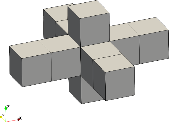 |
| 1 | Ellipsoid | 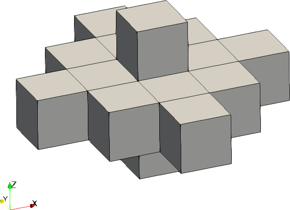 |
| 2 | Cuboid | 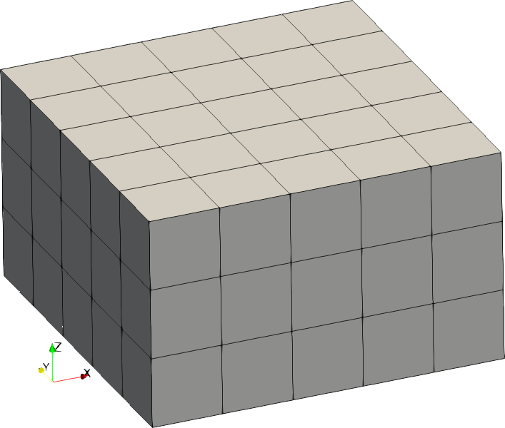 |
If a reference image is provided in input to the method, the Savitzky-Golay filter is anatomically adapted with respect to it. Precisely, in the filter procedure each voxel contribution is weighted according to a Gaussian of standard deviation weight-param applied to the relative contrast with respect to the central voxel.
Other parameters
[parameter]
    output-variance = "example.h5:/var"
output-varianceis the address where the variance evaluated for the electric properties will be written. It must be a group in an .h5 file. The variance of the electric conductivity, if available, will be written in the group as/electric-conductivity; the variance of the relative permittivity, if available, will be written in the group as/relative-permittivity. If omitted, the variance will not be stored (not even evaluated). For the phase-based approximation, the variance is evaluated only with an unwrapped phase input.
Example
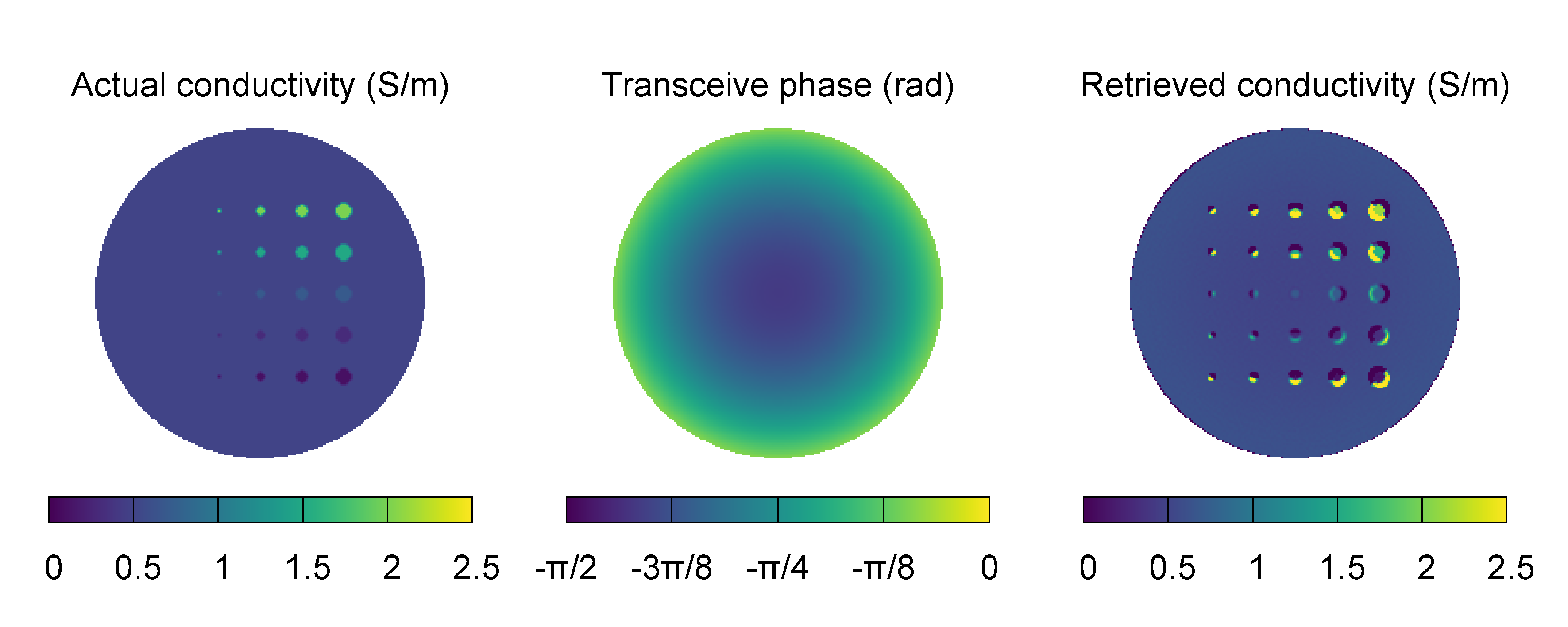
The following configuration file is used to perform the phase-based approximated Helmholtz EPT of a heterogeneous phantom. The input transceive phase has been obtained by simulating the phantom in a birdcage body coil at 64 MHz, that is the Larmor frequency of a 1.5 T scanner.
The configuration file can be downloaded here. The input .h5 file containing the data can be downloaded here.
title = "Example of Helmholtz EPT"
description = "Heterogeneous phantom imaged at 1.5 T. Phase-based approximation."
method = 0

[mesh]
    size = [200, 200, 11]
    step = [1e-3, 1e-3, 1e-3]

[input]
    frequency = 64e6
    tx-channels = 1
    rx-channels = 1
#   tx-sensitivity = 'heterogeneous-phantom-15t.h5:tx_sens'
    trx-phase = 'heterogeneous-phantom-15t.h5:trx_phase'

[output]
    electric-conductivity = 'heterogeneous-phantom-15t-ept-helmholtz.h5:sigma'
#   relative-permittivity = 'heterogeneous-phantom-15t-ept-helmholtz.h5:epsr'

[parameter.savitzky-golay]
    size = [1, 1, 1]
    shape = 0
The retrieved distribution of the electric conductivity is pictured in the following image, together with the expected distribution and the input transceive phase. Because of the hypothesis of local homogeneity of the electric properties that is at the basis of the Helmholtz EPT method, large errors occur at the boundary of the phantom inclusions.